casys/engine · deep dive 4 notebooks

Two Parameters, +22.7pp

The residual connection changed everything.

NB-12NB-14NB-15NB-16

The Problem with Message Passing

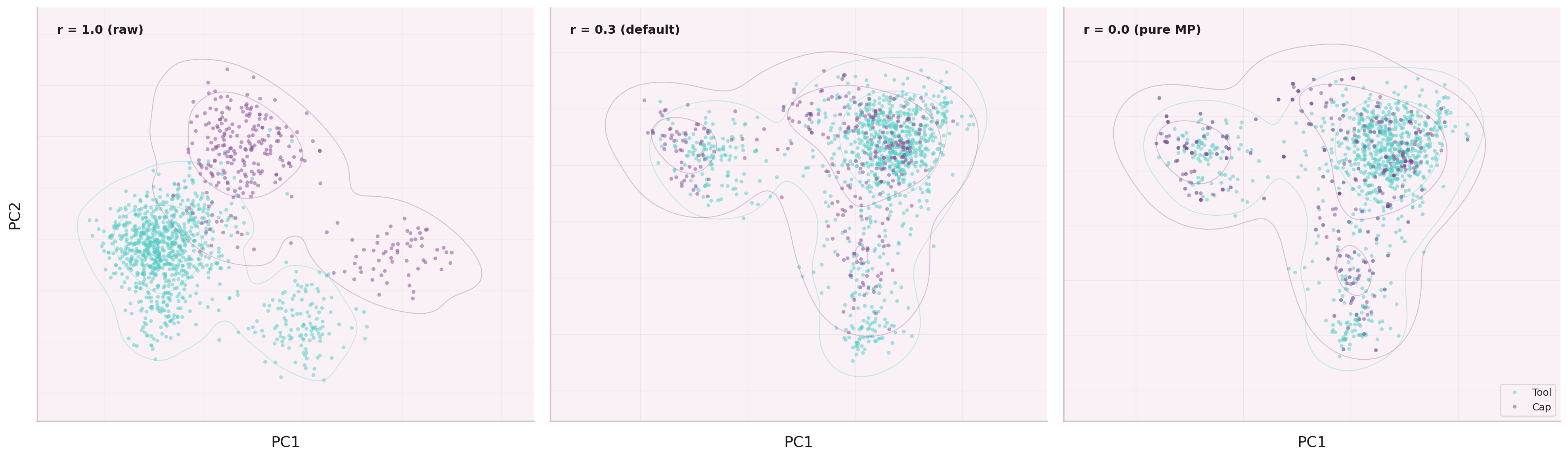
Standard graph neural networks replace each node's embedding with a weighted average of its neighbors. For dense graphs this works well — nodes have many neighbors to average over, producing stable representations.

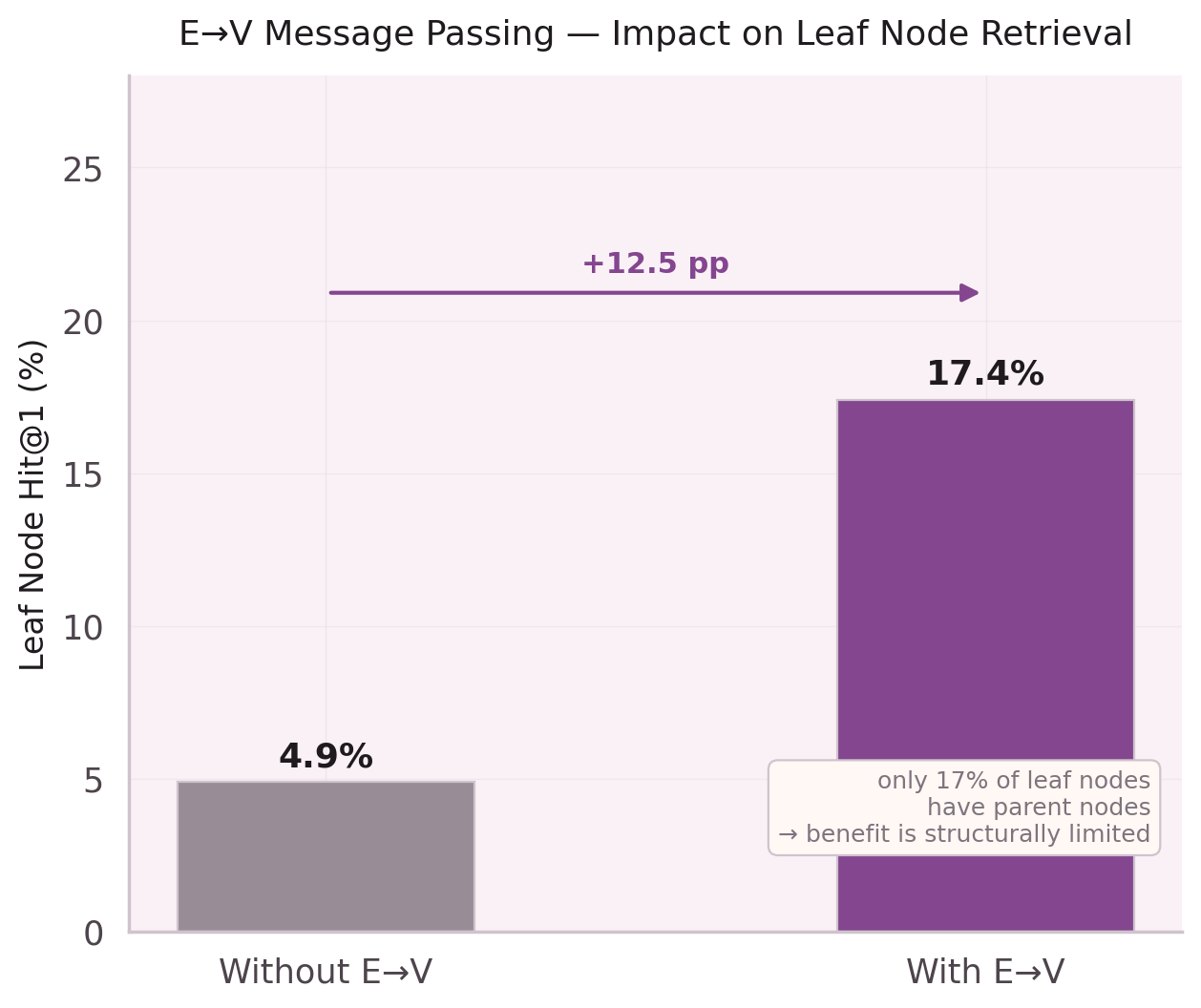
For sparse graphs — like a node co-execution graph where the average node degree is 4.7 — aggregation destroys information. A node with two neighbors becomes an average of those two neighbors, losing its own identity entirely.

Before: standard aggregation

E_new[c] = ELU(Σ α·H')

Leaf nodes lose identity. Hub nodes dominate.

After: vertex-to-edge residual

E_new[c] = ELU(Σ α·H') + γ(n_c)·E[c]

where γ(n) = σ(a·log(n+1) + b) — two learnable parameters

Sparse nodes keep their identity. Dense nodes blend adaptively.

Residual sweep: Hit@1 vs fixed weight r — r=0 dominates every node — **NB-12 · Sweep.** r=0 (pure MP) wins at every single one of 280 nodes tested. No static weight generalizes.

PCA of node embeddings: no residual vs fixed residual vs adaptive gamma — **NB-12 · PCA.** Adaptive γ produces the clearest L0/L1 node separation in PCA space.

The Four Notebooks

The residual was not invented in one step. Four notebooks trace the path from the initial observation (NB-12) to the final parameterization (NB-16).

NB-12 Residual Ablation

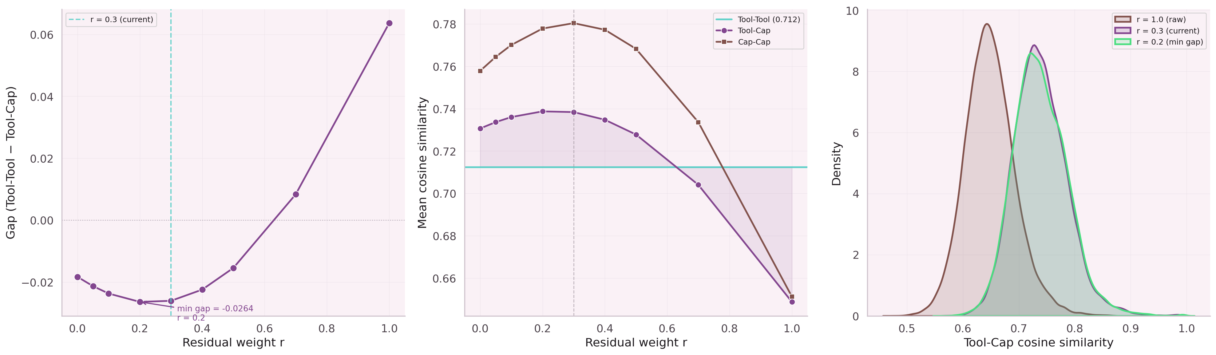
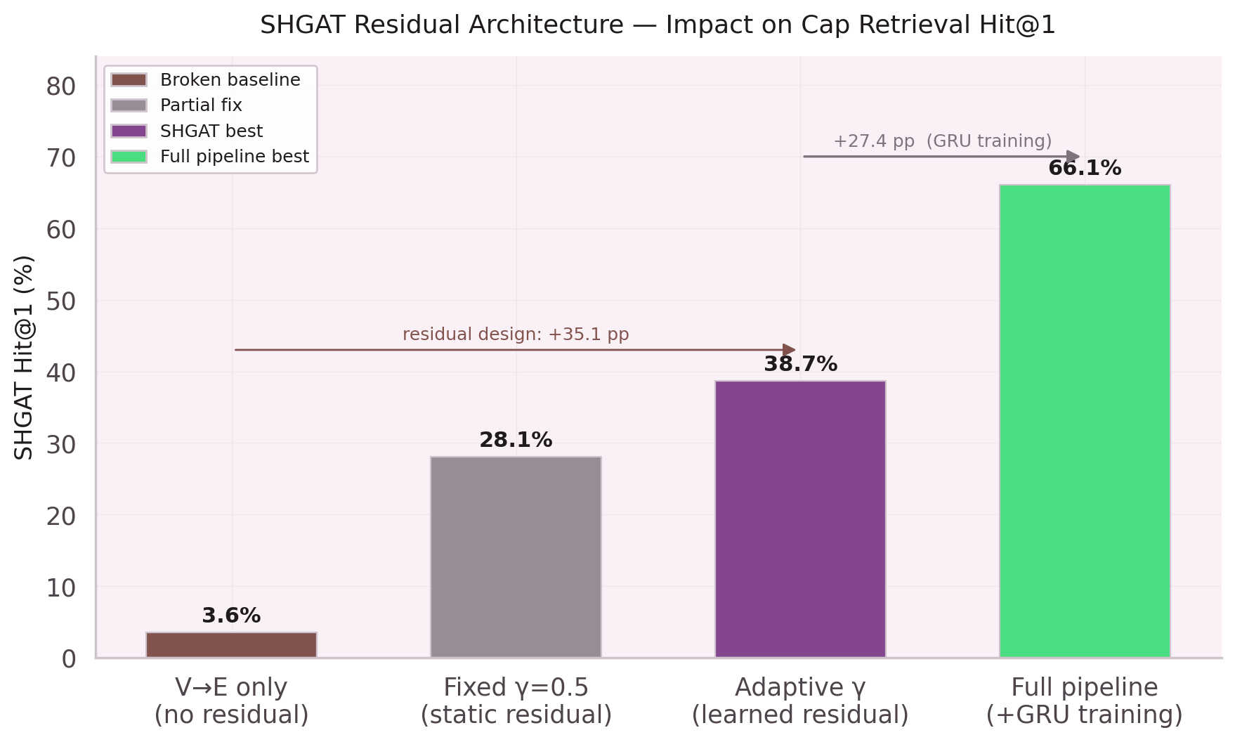
First experiment: add a skip connection with a fixed weight α. Result: α=0.99 is a no-op, α=0.5 collapses representation quality. No static weight works across the full degree distribution.

NB-14 Grid Search on (a, b)

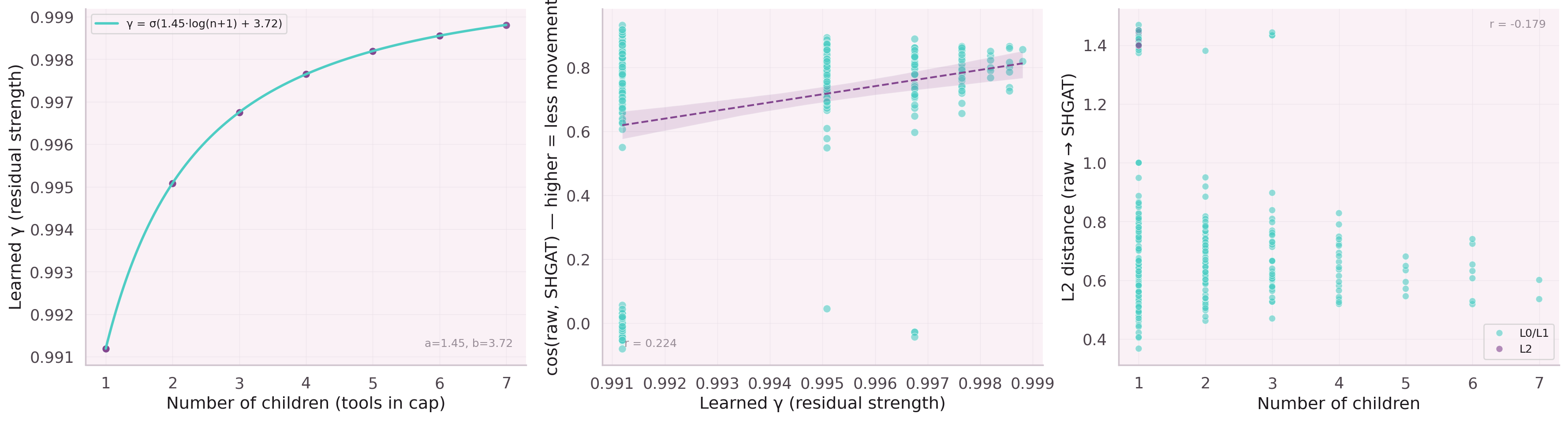
The weight must be a function of degree, not a constant. Grid search over initialization values for a and b. Optimal init: a=−1.0, b=0.5 — γ starts near 0.5 and learns from there.

NB-15 Training Dynamics

Hit@1 at epoch 0: 38.3%. At epoch 10: 59.0% (best checkpoint). Early stop at epoch 12. The residual parameters converge in the first 5 epochs, after which the rest of SHGAT fine-tunes around them.

NB-16 V→E Phase Separation

Final architecture: the residual is applied post-concat-heads in the multi-level orchestrator, at embDim=1024 (not per-head). The V→E code path is separate from the standard forward pass.

V→E propagation alone: Hit@1 collapses to 3.6% — **NB-14 · V→E analysis.** Pure V→E alone: 3.6% Hit@1. Learnable γ recovers to 38.7%. Edges encode co-occurrence, not semantics.

E→V message passing boosts leaf nodes from 4.9% to 17.4% — **NB-15 · E→V impact.** Leaf Hit@1: 4.9% → 17.4%. Only 17% of leaves have parent nodes — limited structural coverage.

Trained adaptive gamma function γ(n) — gate values across node degrees after training — **NB-16 · Trained γ(n).** After training: a=−1.45, b=3.72 → γ≈0.99 for all degrees. The model learned to preserve identity almost entirely.

What the Model Learned

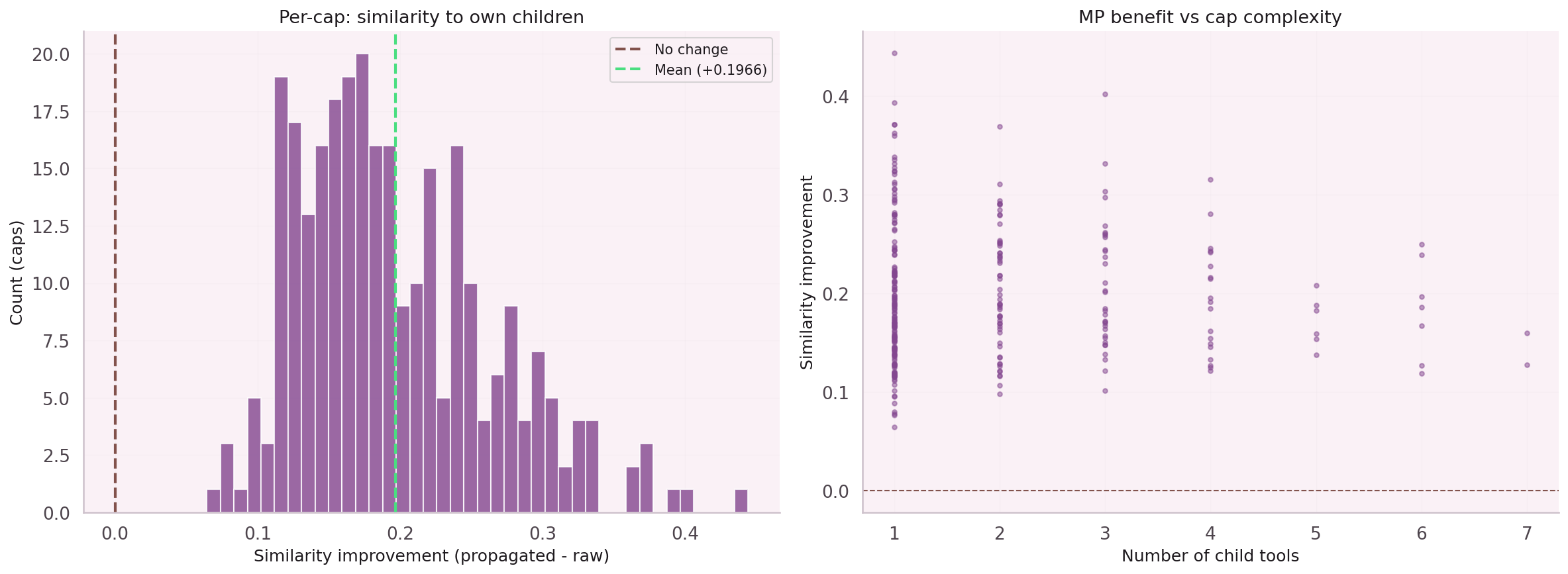
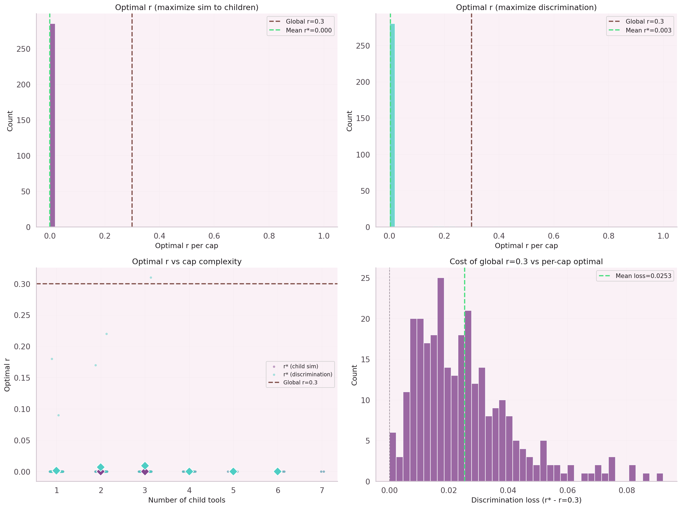
After training, the learned γ(n) function was inspected. Nodes with 1–3 children (sparse leaf nodes) retain ~80% of their original embedding. Hub parent nodes with 10+ children blend down to ~40%.

The model discovered the right tradeoff without being told. The initialization provided a reasonable starting point; the gradient did the rest. Two parameters. Thirty epochs. Twenty-two points.

Per-capability improvement: pure MP vs fixed residual, 280 parent nodes — **NB-12 · Per-cap improvement.** Pure MP (r=0) improves every node over the fixed-residual baseline. No exceptions.

Optimal r distribution across 280 parent nodes — all cluster at r=0 — **NB-12 · Optimal r distribution.** 100% of 280 nodes prefer r=0. The data rejected the fixed-residual hypothesis entirely.