Scoring Tool Relevance Without an LLM
How a 258K-parameter pipeline outperforms embedding similarity for next-node prediction in agentic systems.
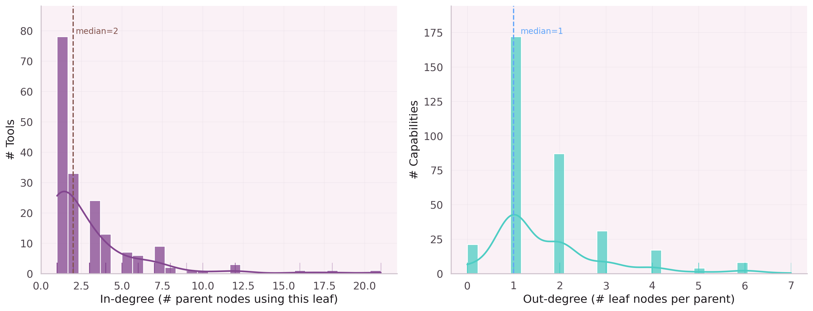
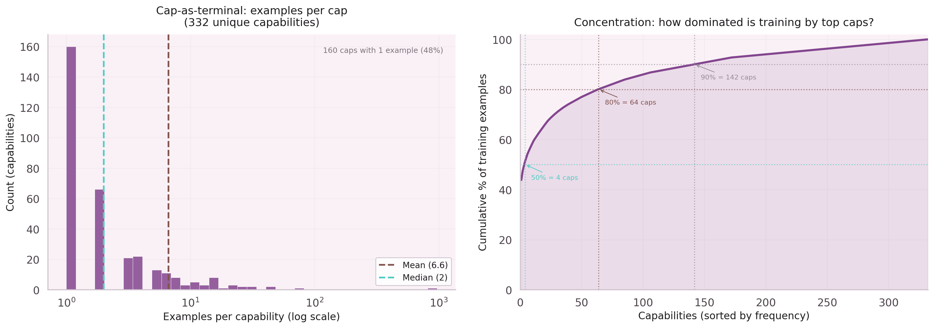
920 Tools, Hubs, and a Long Tail
When an LLM agent has 920 tools available, how does it choose the right one? The standard approach is embedding similarity: embed the user's intent, embed each tool description, find the nearest vectors.
This works for 10 tools. At 920, the graph structure matters. Tools form hierarchies and sequences that pure embeddings cannot capture. The co-execution graph has:
875 edges connect them. Average node degree: 4.7 — a sparse graph where hub parent nodes aggregate many leaf nodes, and the long tail of single-use leaf nodes needs a different treatment than popular hubs.
Chaos vs. Structure
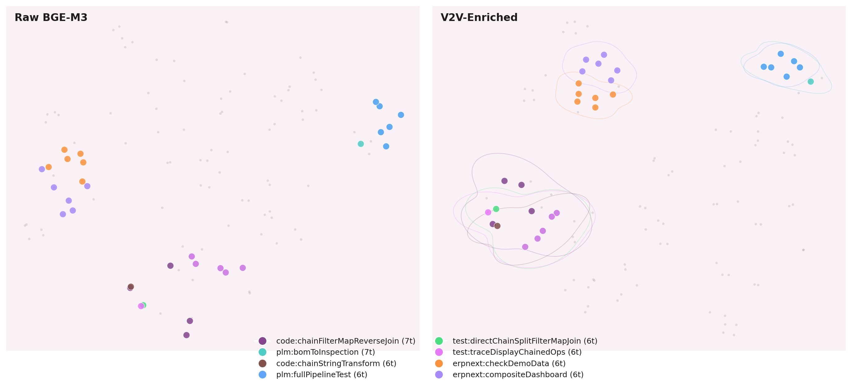
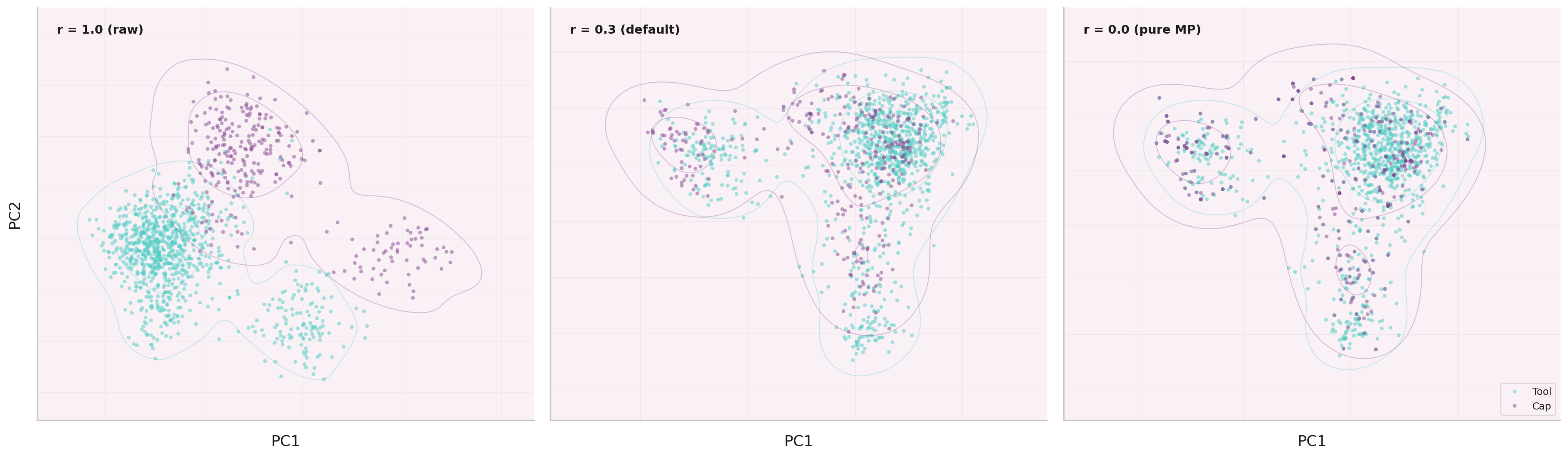
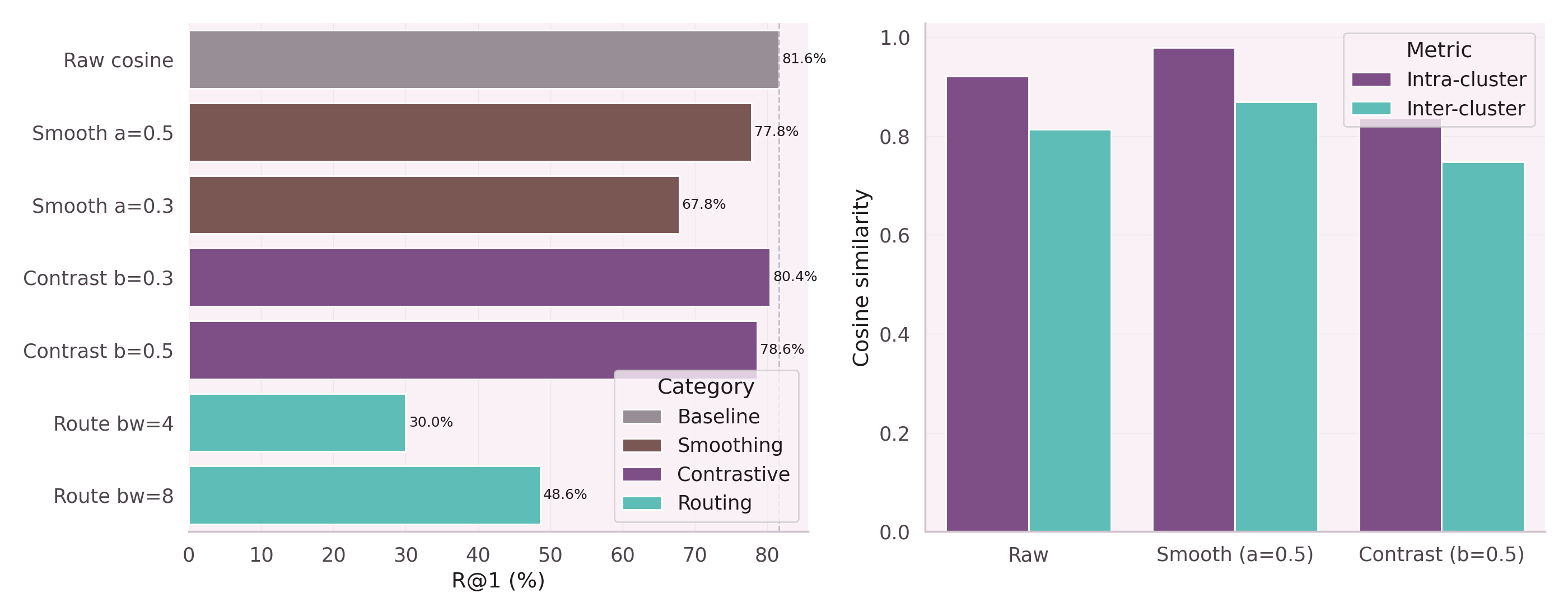
Raw tool embeddings cluster by lexical similarity: tools with
similar descriptions sit near each other, regardless of how they are actually
used together. Two PostgreSQL tools look identical; generate_bom
and query_parts_db look distant despite always executing in sequence.
After SHGAT enrichment, the geometry changes. Tools that co-execute move together. Tools that serve different contexts — even with similar names — are pushed apart.
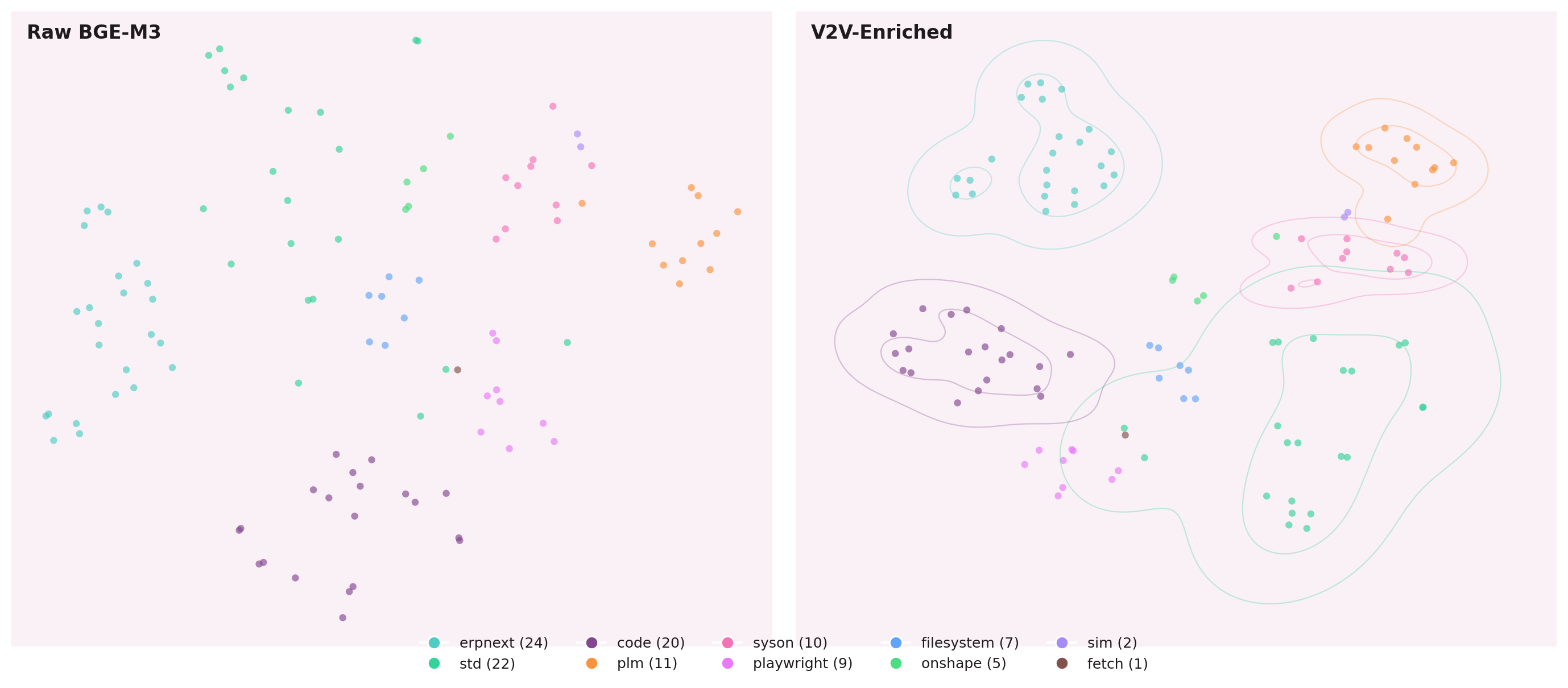
The structure is learned from behavior, not descriptions. Tools that work together move together in embedding space.
Smoothing Kills. Contrastive Discriminates.
Standard message passing averages a node's embedding with its neighbors. On a tool graph, this is lethal: a tool that rarely co-executes with others gets washed into its neighborhood and loses its identity.
The key insight from NB-01: contrastive loss during message passing pushes siblings apart while pulling co-executors together. Smoothing creates uniformity. Contrastive creates discrimination.

Smoothing message passing kills discrimination. Contrastive message passing pushes siblings apart.
Production SHGAT uses InfoNCE contrastive loss with PER (Prioritized Experience Replay) and curriculum scheduling: easy pairs first, hard negatives after the model has learned the basic structure.
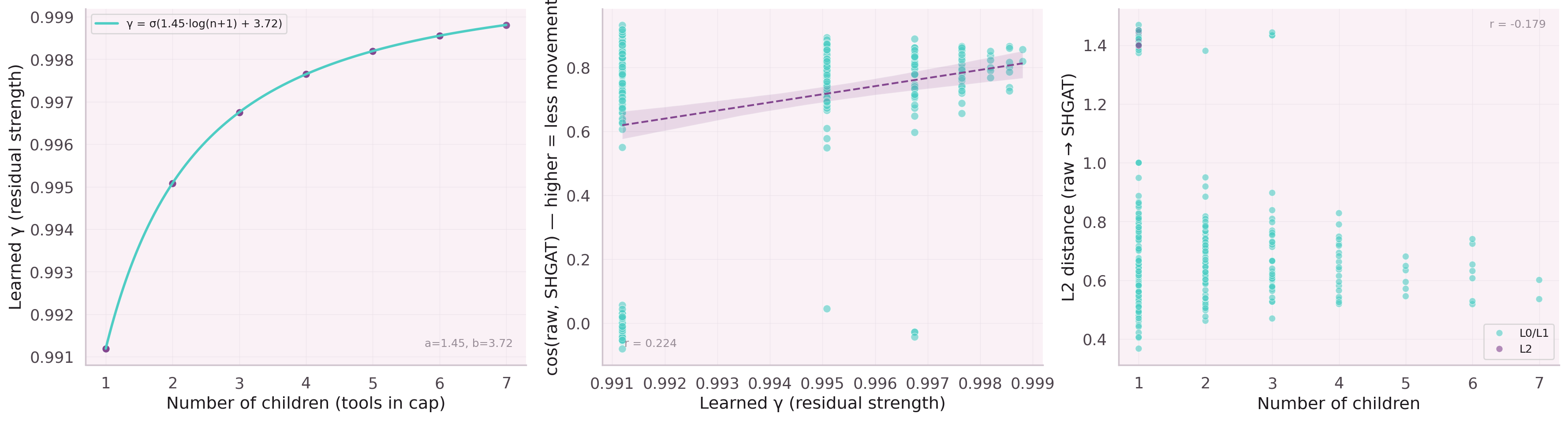
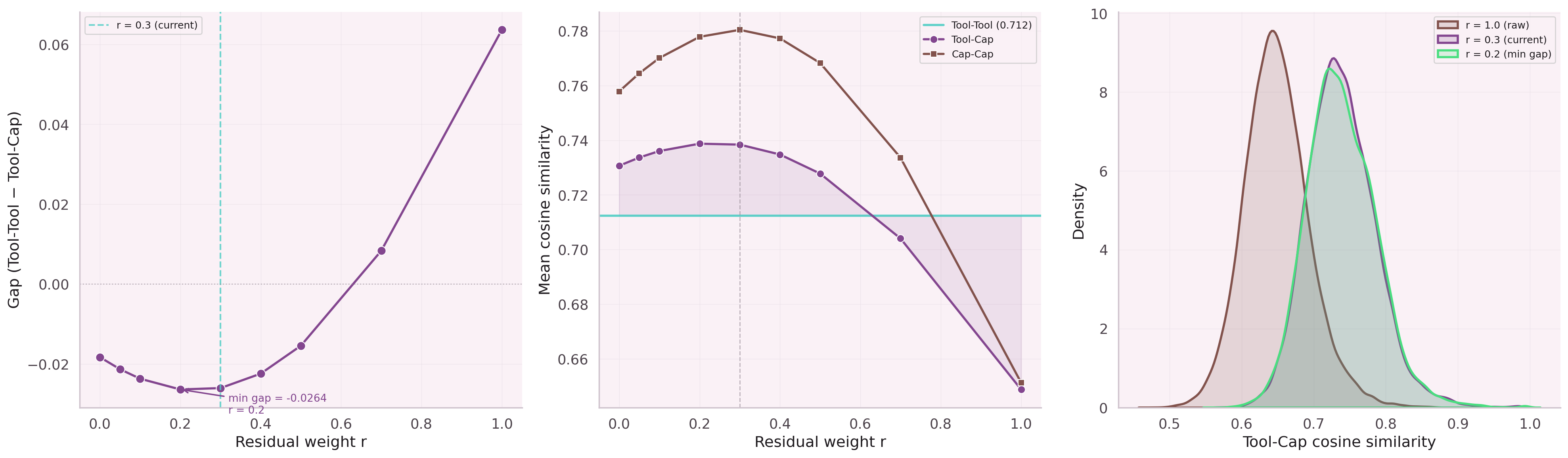
How Much to Keep of the Original Signal?
After message passing, how much of a node's original embedding should survive? Leaf nodes (few connections) should keep most of their identity. Hub parent nodes (many connections) should blend more aggressively with their neighborhood.
The balance is learned, not hand-tuned. Our residual formula:

Training: 1,876 capability-tool pairs · InfoNCE contrastive loss · PER + curriculum · 30 epochs · 7.35M params · ~4 min on CPU
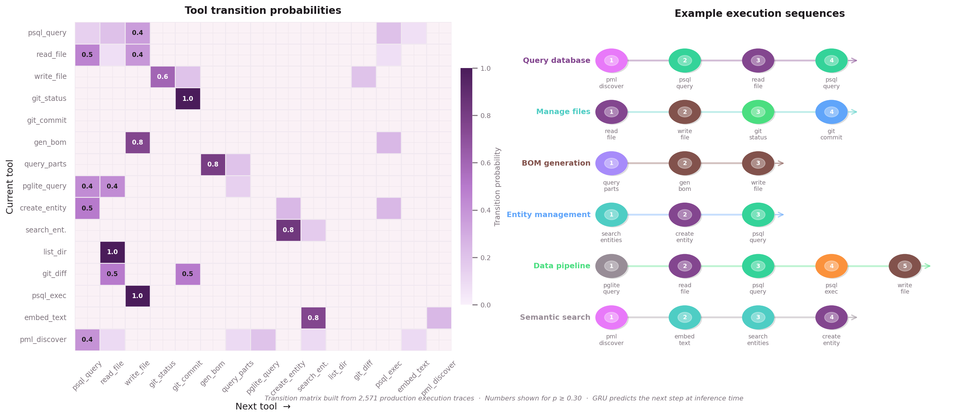
Execution Traces as Directed Sequences
With enriched embeddings from SHGAT, we need a model that predicts which node comes next in a sequence. Execution traces — the ordered list of nodes an agent called to fulfill an intent — are the training signal.
The GRU (Gated Recurrent Unit) is deliberately tiny: 258,000 trainable parameters.
Five inputs at each step:
- SHGAT-enriched embedding of the current node (1024→64 projection)
- Intent embedding (what the user asked for)
- Hierarchy level (L0 / L1 / L2)
- Positional encoding (sequence position)
- Edge features (from the graph)
The hidden state (64-dim GRU) captures execution context. At each step, it predicts over the full vocabulary: 1,165 nodes = 920 leaf nodes + 245 parent nodes.
Why Not an LLM?
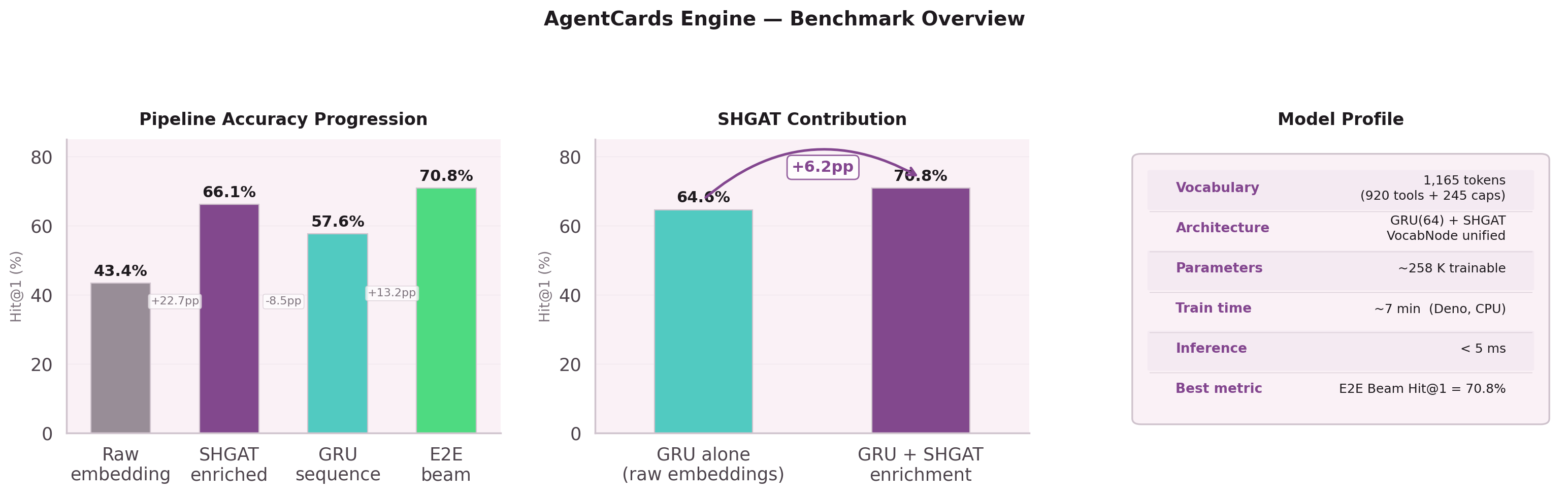
Component Results
Training: 2,571 execution traces · frequency capping (30/cap, FPS) · early stopping ep 48 · ~3 min on CPU
The Full Pipeline
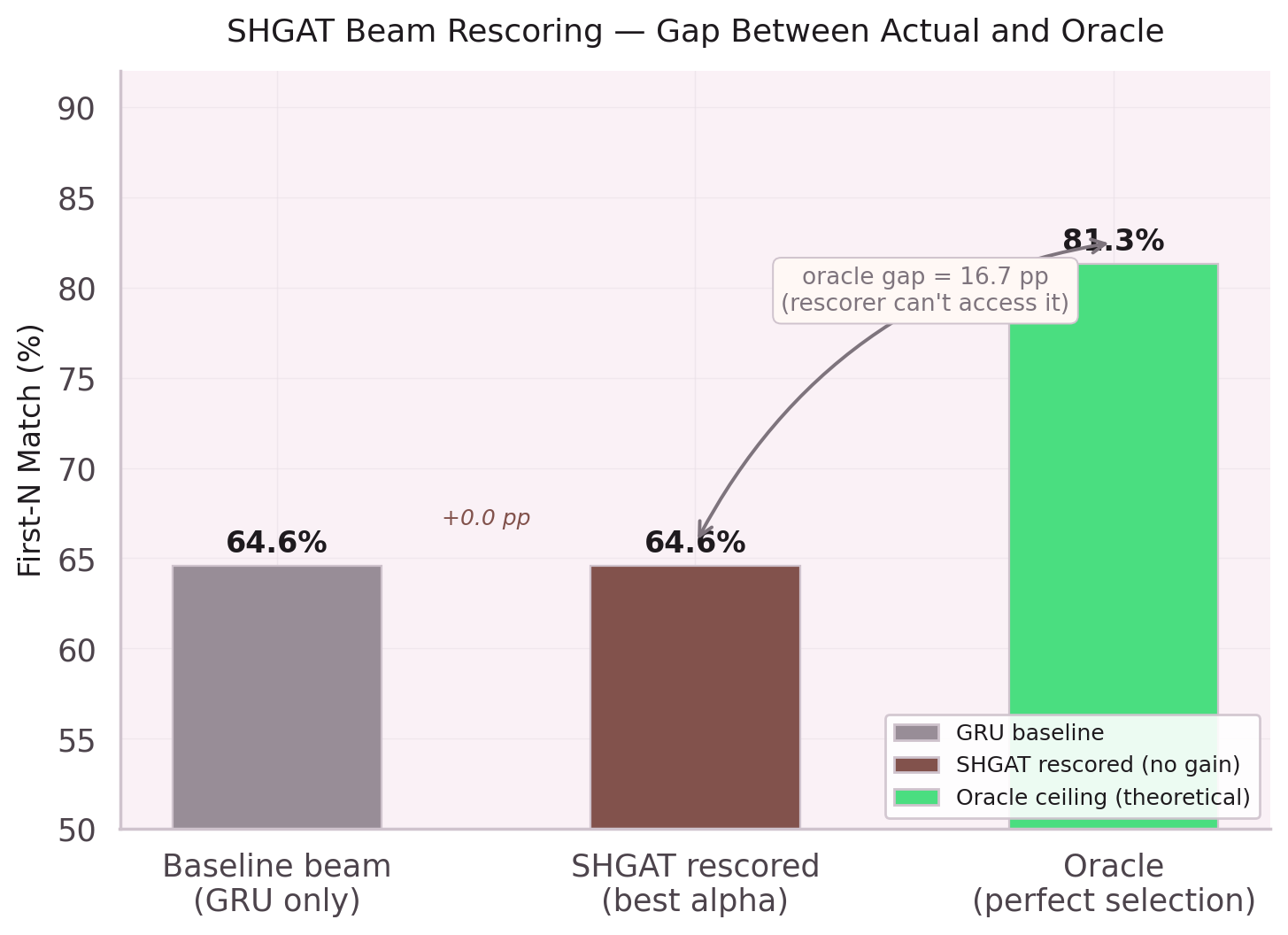
The real test is end-to-end: given an intent, predict the full node sequence using beam search (width 5) with length normalization.
| Configuration | First-N Accuracy | Δ |
|---|---|---|
| GRU alone (raw embeddings) | 64.6% | baseline |
| GRU + SHGAT enrichment | 70.8% | +6.2pp |
For 7 out of 10 user intents, the predicted node sequence starts with the correct nodes.
The entire SHGAT + GRU pipeline completes inference in under 5ms. No GPU. No API dependency. 258K parameters running on any device.
What Remains Open
- Vocabulary growth — adding leaf nodes requires retraining. No online learning yet.
- Cold start — new leaf nodes with zero traces get no structural benefit.
- Cap-frequency tradeoff — aggressive capping helps parent node prediction but hurts leaf node prediction.
- Canonicalization — 28 duplicate toolset groups dilute softmax (+25.7pp when canonicalized, not yet in prod).
24 Notebooks of Evidence
Each design decision above is backed by ablation studies, visualizations, and failure analysis. Five deep dive tracks cover the full research arc.
Data Quality Odyssey
The data is the real problem
Nodes All The Way Down
Unified vocabulary, recursive prediction
Two Parameters, +22.7pp
The residual connection changed everything
What Didn't Work
Five failed approaches, equally important
Scaling & Retrieval
Before the pipeline: foundational theory
Based on 24 Jupyter notebooks of experiments, January–February 2026.